TEA-seq: topic modeling of a RNA + ATAC + protein PMBCs#
This tutorial runs topomics (MultimodalAmortizedLDA) on a tri-modal
TEA-seq dataset (paired single-cell
RNA, ATAC, and surface protein). It shows how to:
load the data and prepare the
MuData,(training is shown for reference but commented out) — we load a model from disk,
extract the cell-topic distribution θ,
inspect the top features per topic in each modality,
visualize topics on a UMAP, and
summarize topic usage per cell type.
Configuration#
Just some utilities to load a pre-trained model for this example
from pathlib import Path
import yaml


def load_config():
    """Load the git-ignored config.yml holding private dataset/model paths.

    Copy ``config.example.yml`` to ``config.yml`` and fill in your paths.
    """
    for p in (Path("config.yml"), Path("../config.yml"), Path("examples/config.yml")):
        if p.exists():
            return yaml.safe_load(p.read_text())
    raise FileNotFoundError("config.yml not found. Copy config.example.yml to config.yml and edit it.")


CONFIG = load_config()

cfg = CONFIG["datasets"]["teaseq"]
Imports#
import numpy as np
import pandas as pd
import scanpy as sc
import muon as mu
import matplotlib.pyplot as plt

from topomics import MultimodalAmortizedLDA

sc.settings.verbosity = 1
MODALITY_ORDER = ["rna", "atac", "prot"]
Load data#
The MuData holds three modalities, each with raw counts in layers["counts"].
We restrict RNA/ATAC to highly variable features exactly as the model was trained,
and binarize ATAC.
mdata = mu.read_h5mu(cfg["data"])

sc.pp.highly_variable_genes(mdata.mod["rna"], n_top_genes=2000, flavor="seurat_v3", layer="counts")
mdata.mod["rna"] = mdata.mod["rna"][:, mdata.mod["rna"].var["highly_variable"]].copy()

sc.pp.highly_variable_genes(mdata.mod["atac"], n_top_genes=10000, flavor="seurat_v3", layer="counts")
mdata.mod["atac"] = mdata.mod["atac"][:, mdata.mod["atac"].var["highly_variable"]].copy()

# ATAC uses a Bernoulli likelihood -> encode peaks as presence/absence (0/1).
_atac = mdata.mod["atac"]
_atac.layers["counts"] = (_atac.layers["counts"] > 0).astype("float32")

mdata.update()
mdata
MuData object with n_obs × n_vars = 5805 × 12046
  obs:	'sample', 'well', 'leiden_multiplex', 'leiden_mofa', 'celltypist_label', 'celltypist_confidence'
  var:	'highly_variable', 'gene_ids', 'feature_types', 'genome', 'interval'
  uns:	'leiden', 'leiden_mofa', 'leiden_mofa_colors', 'mofa', 'umap'
  obsm:	'X_mofa', 'X_mofa_umap', 'X_umap'
  varm:	'LFs'
  obsp:	'mofa_connectivities', 'mofa_distances'
  3 modalities
    rna:	5805 x 2000
      obs:	'n_genes_by_counts', 'total_counts', 'total_counts_mt', 'pct_counts_mt', 'leiden', 'celltypist_label', 'celltypist_confidence'
      var:	'gene_ids', 'feature_types', 'genome', 'interval', 'mt', 'n_cells_by_counts', 'mean_counts', 'pct_dropout_by_counts', 'total_counts', 'highly_variable', 'means', 'dispersions', 'dispersions_norm', 'mean', 'std', 'highly_variable_rank', 'variances', 'variances_norm'
      uns:	'hvg', 'leiden', 'leiden_colors', 'leiden_multiplex_colors', 'log1p', 'neighbors', 'pca', 'rna:leiden_colors', 'umap'
      obsm:	'X_pca', 'X_umap'
      varm:	'PCs'
      layers:	'counts', 'lognorm'
      obsp:	'connectivities', 'distances'
    atac:	5805 x 10000
      obs:	'n_fragments', 'n_duplicate', 'n_mito', 'n_unique', 'altius_count', 'altius_frac', 'gene_bodies_count', 'gene_bodies_frac', 'peaks_count', 'peaks_frac', 'tss_count', 'tss_frac', 'barcodes', 'cell_name', 'well_id', 'chip_id', 'batch_id', 'pbmc_sample_id', 'DoubletScore', 'DoubletEnrichment', 'TSSEnrichment', 'n_genes_by_counts', 'total_counts', 'n_counts', 'leiden'
      var:	'gene_ids', 'feature_types', 'genome', 'interval', 'n_cells_by_counts', 'mean_counts', 'pct_dropout_by_counts', 'total_counts', 'highly_variable', 'means', 'dispersions', 'dispersions_norm', 'mean', 'std', 'highly_variable_rank', 'variances', 'variances_norm'
      uns:	'hvg', 'leiden', 'leiden_colors', 'log1p', 'neighbors', 'pca', 'umap'
      obsm:	'X_pca', 'X_umap'
      varm:	'PCs'
      layers:	'counts', 'lognorm'
      obsp:	'connectivities', 'distances'
    prot:	5805 x 46
      obs:	'total_counts'
      var:	'highly_variable'
      uns:	'neighbors', 'pca', 'umap'
      obsm:	'X_pca', 'X_umap'
      varm:	'PCs'
      layers:	'counts'
      obsp:	'connectivities', 'distances'
Register the MuData with topomics#
mdata_setup, modality_names, feat_counts = MultimodalAmortizedLDA.setup_mudata(
    mdata,
    modality_order=MODALITY_ORDER,
    layers="counts",  # remember to specify the layer the data is stored in
    # or the model will select .X
)
print("modalities:", modality_names, "| feature counts:", feat_counts)
modalities: ['rna', 'atac', 'prot'] | feature counts: [2000, 10000, 46]
Training (for reference — skipped here)#
This is how the model was trained. In this tutorial we assume that we have already trained the model. Uncomment to train from scratch (needs a GPU and a few minutes).
# model = MultimodalAmortizedLDA.from_mudata(
#     mdata,
#     modality_order=MODALITY_ORDER,
#     layers="counts",
#     n_topics=20,
#     likelihoods=["gamma_poisson", "bernoulli", "gamma_poisson"],
#     cell_topic_prior=1 / 20,
# )
# model.train(max_epochs=200, batch_size=256)
# model.save(cfg["model"], overwrite=True)
Load the trained model#
load needs an AnnData with the same feature layout used at training time.
setup_mudata already stored that flattened AnnData under
mdata.uns["_flattened_ann_data"], so we reuse it directly.
adata_flat = mdata_setup.uns["_flattened_ann_data"]
model = MultimodalAmortizedLDA.load(cfg["model"], adata=adata_flat)
model
INFO     File
         /data/omics_topic_models/teaseq_2.0/logistic_normal_moe_cell/prior_logistic_normal_weight_cell_learnable_d
         isp_pergene/model/model.pt already downloaded
Epoch 1/1000:   0%|          | 1/1000 [00:00<01:06, 14.96it/s, v_num=1]
Epoch 1/1000:   0%|          | 1/1000 [00:00<01:11, 14.01it/s, v_num=1]
Training status: Trained
Cell-topic distribution θ#
get_latent_representation returns the (cells x topics) matrix. With
return_dataframe=True we get topic-labeled columns indexed by cell.
Notice that in principle we are approximating a posterior distribution for each point, but in this case we simply take the average, without sampling.
theta = model.get_latent_representation(batch_size=mdata.n_obs, return_dataframe=True)
print("theta shape:", theta.shape)
theta.head()
theta shape: (5805, 10)
| topic_0 | topic_1 | topic_2 | topic_3 | topic_4 | topic_5 | topic_6 | topic_7 | topic_8 | topic_9 | |
|---|---|---|---|---|---|---|---|---|---|---|
| AAACAGCCAATTAAGG-1 | 0.174442 | 0.007398 | 0.153438 | 0.166352 | 0.180219 | 0.010132 | 0.153502 | 0.121624 | 0.007727 | 0.025167 |
| AAACAGCCACCCTCAC-1 | 0.180788 | 0.009597 | 0.152533 | 0.181792 | 0.188855 | 0.006604 | 0.197608 | 0.050097 | 0.011024 | 0.021102 |
| AAACAGCCAGCTCAAC-1 | 0.156339 | 0.011893 | 0.189569 | 0.163712 | 0.171924 | 0.010939 | 0.183209 | 0.067951 | 0.010783 | 0.033682 |
| AAACAGCCAGTATGTT-1 | 0.025995 | 0.181268 | 0.163482 | 0.025100 | 0.016614 | 0.011691 | 0.166433 | 0.122099 | 0.281996 | 0.005322 |
| AAACAGCCATCAATCG-1 | 0.043409 | 0.155075 | 0.179874 | 0.050378 | 0.031177 | 0.014819 | 0.222904 | 0.079410 | 0.211628 | 0.011327 |
Top features per topic#
def top_features_per_topic(model, mdata, modality_order, n_top=10, n_samples=2000):
    """Return a dict {modality: DataFrame(topic x rank) of feature names}.

    ``model.module.topic_by_feature()`` gives E[phi_{k,m}] as a dict
    {modality_index: tensor (n_topics, n_features_m)}; we map columns back to
    the per-modality ``var_names``.
    """
    import numpy as np

    tbf = model.module.topic_by_feature(n_samples=n_samples)
    out = {}
    for m, mod in enumerate(modality_order):
        phi = np.asarray(tbf[m])  # (n_topics, n_features_m)
        var_names = np.asarray(mdata.mod[mod].var_names)
        rows = {}
        for k in range(phi.shape[0]):
            top_idx = np.argsort(phi[k])[::-1][:n_top]
            rows[f"topic_{k}"] = var_names[top_idx]
        out[mod] = pd.DataFrame(rows).T
        out[mod].columns = [f"rank_{i + 1}" for i in range(n_top)]
    return out


top = top_features_per_topic(model, mdata, MODALITY_ORDER, n_top=10)
print("Top RNA genes per topic:")
top["rna"].head()
Top RNA genes per topic:
| rank_1 | rank_2 | rank_3 | rank_4 | rank_5 | rank_6 | rank_7 | rank_8 | rank_9 | rank_10 | |
|---|---|---|---|---|---|---|---|---|---|---|
| topic_0 | CD28 | TRAT1 | BICDL1 | ICOS | TNFAIP3 | ZFPM1 | PBX4 | CDC14A | GATA3 | BCL11B |
| topic_1 | HLA-DRB1 | CDK14 | HLA-DRB5 | GRK3 | MYO1E | HLA-DRA | LYN | TBC1D9 | TRIO | HLA-DPA1 |
| topic_2 | WWOX | ABCA6 | ATP8A1 | FBXL17 | AC010996.1 | KCNQ5 | SMYD3 | GMDS-DT | GNPTAB | CFAP299 |
| topic_3 | FHIT | IGF1R | LEF1 | NRCAM | TSHZ2 | NDFIP1 | MLLT3 | LRRC7 | MAML2 | FAM117B |
| topic_4 | PRKCA | BCL11B | LEF1 | TSHZ2 | PLCL1 | CAMK4 | APBA2 | CMTM8 | LEF1-AS1 | CD247 |
top["prot"].head() # top proteins per topic
| rank_1 | rank_2 | rank_3 | rank_4 | rank_5 | rank_6 | rank_7 | rank_8 | rank_9 | rank_10 | |
|---|---|---|---|---|---|---|---|---|---|---|
| topic_0 | prot:CD127 | prot:CD278 | prot:CD3 | prot:CD27 | prot:CD95 | prot:CD4 | prot:CD45RO | prot:CD279 | prot:TCR-a/b | prot:CD80 |
| topic_1 | prot:HLA-DR | prot:CD123 | prot:CD39 | prot:CD71 | prot:FceRI | prot:TCR-g/d | prot:IgM | prot:CD10 | prot:CD40 | prot:CD86 |
| topic_2 | prot:CD45RA | prot:CD38 | prot:CD197 | prot:IgG1-K-Isotype-Control | prot:CD24 | prot:TCR-Va24-Ja18 | prot:CD16 | prot:CD269 | prot:TCR-g/d | prot:TCR-a/b |
| topic_3 | prot:CD4 | prot:CD27 | prot:CD3 | prot:CD197 | prot:CD8a | prot:TCR-a/b | prot:CD45RA | prot:CD278 | prot:CD127 | prot:CD24 |
| topic_4 | prot:CD3 | prot:CD27 | prot:CD4 | prot:CD278 | prot:CD197 | prot:TCR-a/b | prot:CD127 | prot:CD80 | prot:CD304 | prot:IgG1-K-Isotype-Control |
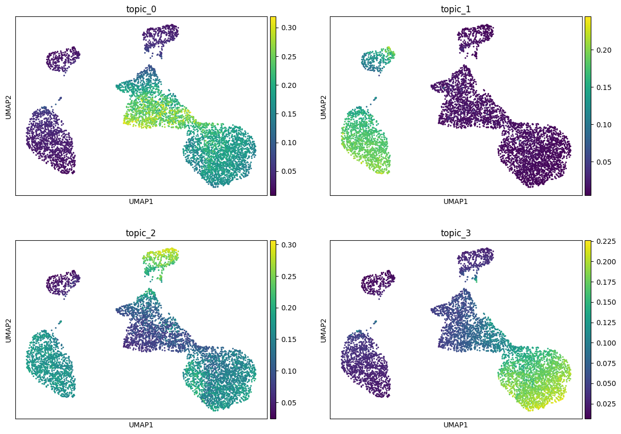
Visualize topics on a UMAP#
Topic modeling can be seen as a special kind of dimensionality reduction, so we can build a UMAP directly in topic space and check that the result is plausible. We first colour the embedding by a few topic weights, then by the annotated cell type. Notice that the distance we use for the topic space is the Hellinger distance (https://en.wikipedia.org/wiki/Hellinger_distance) which can be conventiently calculated by taking the sqrt of the \(\theta\)s and then compute the Euclidean distance.
topic_adata = sc.AnnData(theta.values)
topic_adata.obs_names = theta.index
topic_adata.obs[theta.columns] = theta.values
topic_adata.obsm["theta_sqrt"] = np.sqrt(theta.values)

sc.pp.neighbors(topic_adata, use_rep="theta_sqrt", n_neighbors=15)
sc.tl.umap(topic_adata)

show_topics = list(theta.columns[:4])
sc.pl.umap(topic_adata, color=show_topics, ncols=2, cmap="viridis", show=True)
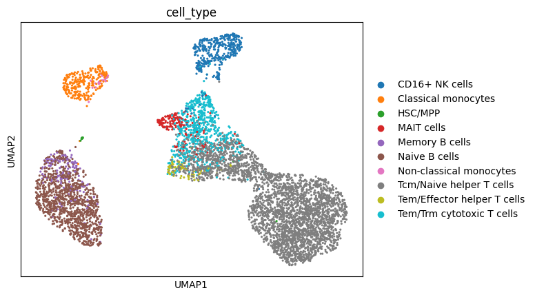
# UMAP of the topic space, coloured by annotated cell type.
# (celltype_key comes from config.yml; here: "celltypist_label")
ct_key = cfg["celltype_key"]
topic_adata.obs["cell_type"] = mdata.mod["rna"].obs[ct_key].astype("category").values
sc.pl.umap(topic_adata, color="cell_type", show=True)
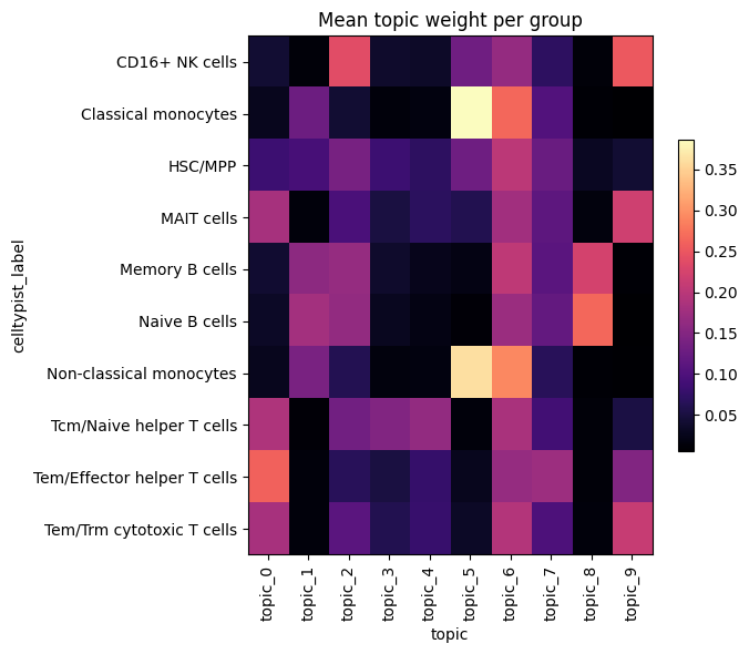
Topic usage per cell type#
Mean topic weight within each cell type highlights which topics mark which
populations. We use the celltype_key from the config (falling back to a leiden
clustering of the topic space if it is missing).
def topic_proportions_by_group(theta_df, groups):
    """Mean topic weight per group (e.g. cell type or cluster)."""
    df = theta_df.copy()
    df["__group__"] = pd.Series(list(groups), index=theta_df.index)
    return df.groupby("__group__").mean()


ct_key = cfg.get("celltype_key")
rna_obs = mdata.mod["rna"].obs

groups = rna_obs[ct_key].values
group_name = ct_key
prop = topic_proportions_by_group(theta, groups)

fig, ax = plt.subplots(figsize=(0.5 * theta.shape[1] + 2, 0.4 * prop.shape[0] + 2))
im = ax.imshow(prop.values, aspect="auto", cmap="magma")
ax.set_xticks(range(prop.shape[1]))
ax.set_xticklabels(prop.columns, rotation=90)
ax.set_yticks(range(prop.shape[0]))
ax.set_yticklabels(prop.index)
ax.set_xlabel("topic")
ax.set_ylabel(group_name)
ax.set_title("Mean topic weight per group")
fig.colorbar(im, ax=ax, shrink=0.6)
plt.tight_layout()
plt.show()